반응형
itutorial - Discrete Fourier Transform (DFT) or also called Discrete Fourier Transform is a technique in mathematics for changing a sequence of values or a certain sequence of discrete values in a certain period in the time domain to the frequency domain. DFT aims to convert continuous (analog) signal values into discrete values so that they can be processed or calculated digitally using a microcontroller or computer.
When the author was still in college, DFT was one of the lecture materials that was difficult and complicated, and even after studying, he still didn't pass the exam and had to repeat it. Then the author tries to understand DFT not from the formula and how to solve it, but tries to understand the meaning conveyed by the DFT formula, and finally the author succeeds in understanding the meaning of the DFT formula.
DFT is not a difficult formula and is relatively easy to understand and is important to learn, especially for anyone who has a hobby of electronics or is involved in the world of electronics, so with this blog the author shares experiences on how to understand DFT so that it can be used in real life (not just mathematical formula only).
DFT is very important for basic digital signal processing. One basic example of the application of DFT in the field of electronics is to determine voltage, electrical frequency and its disturbances (harmonics), power factor (cos fi) and electrical power consumption through DFT calculations carried out by a microcontroller or computer.
In general, DFT can do the following things:
Converts discrete signal values in the time domain to discrete values in the frequency domain.
Signals in the time domain can only show one signal which may have an irregular shape. This irregular shape (not purely sinusoidal) indicates that there are other signals with different frequencies and perhaps also different amplitudes or magnitudes that interfere with the sinusoidal signal as shown in Figure 1.
 | |
|
Figure 1 shows that a sinusoidal signal with fundamental frequency f 1 is disturbed by 2 signals f 2 and f 3 resulting in a signal that looks like an image of f t with an irregular shape which looks similar to the signal f 1 but the shape is irregular.
The thing that needs to be understood in DFT is that a continuous signal or analog signal in the time domain needs to be converted first into a discrete signal in the time domain where the value is taken at a certain point in a signal over a certain time which is generally often referred to as a sample.
DFT is able to determine the magnitude of interfering frequencies in a signal, or is able to determine the magnitude of many frequencies in a signal, which is difficult to do in the time domain.
The results of DFT calculations on the f t signal in Figure 1 can distinguish or separate all the frequencies in the f t signal by displaying the spectrum of each signal as in Figure 2.
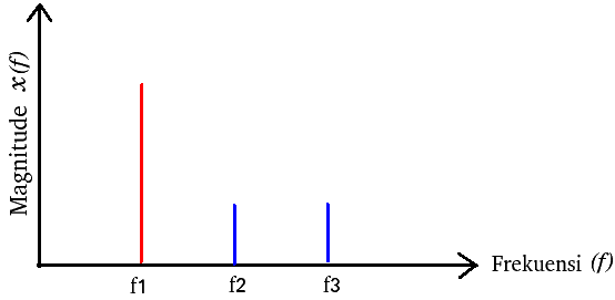 |
| Figure 2. Signal spectrum resulting from DFT calculations |
f 1 has a lower frequency than f 2 but has a greater magnitude than the frequency signals f 2 and f 3 . Meanwhile, the signal spectrum f 2 has a higher frequency than the signal f 1 but lower than the frequency of the signal f 3 . The magnitude of the signals f 2 and f 3 is the same and smaller than the magnitude of the signal f 1 .
From the explanation of Figures 1 and 2, it can be concluded that DFT can change signal variables in the time domain into variables in the frequency domain so that an irregular signal in the time domain can be known at all the frequencies that make up the irregular signal. Signal variables in the frequency domain vary in magnitude , angle (phase) and frequency.
Fourier Series ( Fourier Series )
In mathematics and especially for those of you who study theoretical electronics, you have generally read or heard the term Fourier Series which is generally written as follows:

The meaning of the Fourier Series above can generally be written as follows:
At a certain t value , the Fourier Series above states whether or not the magnitude of a signal is at the lowest frequency value up to the nth frequency ( high frequency).
The Fourier series above can be simplified in writing as follows:

Where the theoretical value of N is infinite. In calculations for applications used in real life it is necessary to limit it to a certain value of N.
A 0 represents the magnitude value when the frequency is 0 or can be said to be the amplitude of the dc component of a signal. Then the next number after A 0 is to express the magnitude of the signal when the frequency is 1 times, 2 times, 3 times up to the nth frequency , where each magnitude value in the sin ( B n ) and cos ( A n ) functions at a certain frequency is added up. To add up all the magnitudes above, this cannot be done using ordinary addition, but by adding each magnitude vector to the sin and cos functions which are generally written in the form of complex numbers and then looking for the resultant.
A n is a coefficient of the cos function or it could be said to be the maximum magnitude of the sin function . To get this value, you need to integrate the cos function at a certain n value . B n is the coefficient of the sin function or can be assumed to be the maximum magnitude of the sin function , and to get this value it is necessary to integrate the value of the sin function at a certain n value .
This DFT material does not discuss how to find the coefficients A n and B n because the focus is on understanding DFT. In DFT, a sinusoidal signal is assumed to be the result of the sum of the cos function signal with maximum magnitude A n and the sin function with maximum magnitude B n .
For a more detailed explanation of DFT, you need to understand the explanation of the addition of the sin and cos functions which are generally written in the form of complex numbers which are explained in the material below.
Basic Signal Functions
The fundamental thing for understanding DFT is to understand the basic signal theory used in DFT. A simple example of the function of a signal is shown in Figure 3.
 |
| Figure 3. Illustration of the signal function with period x |
Figure 3 above shows 3 signal functions of different frequencies with the same magnitude . One signal vibration or wave in one period has one peak and one valley, two vibrations means it has two peaks and two valleys and so on so that the signal function in Figure 3 can be described as follows:
- A signal with the function f(x) = A sin x means that the signal in one period x only has one wave vibration with a maximum magnitude of A.
- A signal with the function f(x) = A sin 2x means that in one period x has 2 wave vibrations or signals with a maximum signal magnitude of A.
- A signal with the function f(x) = A sin 3x means that in one period x has 3 wave vibrations or signals with a maximum signal magnitude of A.
After understanding the meaning of the basic signal function above, the variable x is generally replaced with t because the function is related to time and frequency, so the function above can be written as follows:

The meaning of the equation above is a signal function f
Frequency can also be written in the form of the value 1/T which means the number of rotations or vibrations during one period T. So the function f
From the explanation of the signal illustration in Figure 3, the signal in function of time is shown in Figure 4.
 |
| Figure 4. Illustration of signals in function of time |
If converted into a sentence, the function of the signal above can be explained as follows:
- f
- f
- f
DFT Magnitude
In DFT theory, a function of a signal can be written in the form of a complex number consisting of a real component and an imaginary component . With real and imaginary values , you can find the magnitude value which can be analogous to the amplitude of a signal at a certain frequency, besides that you can also find out the phase of a signal.
The basic understanding of writing signal functions in complex form can be seen in Figure 5.
 |
| Figure 5. Illustration of real and imaginary components in a sinusoidal signal |
A signal with function f

Figure 5 also shows a phasor diagram which states that A s is an imaginary component vector with a maximum value of 1j or often written just j . Meanwhile, A c is a vector of real components whose maximum magnitude is the same as the maximum value of the cos function, namely 1, so that the signal function in complex numbers can be written as follows:

From Figure 5 it can be seen that when the wave or signal moves towards the t axis, the real and imaginary resultant vectors form an angle θ where the resultant moves counterclockwise which causes the positive (+) sign on the imaginary component of the signal function to change to negative (-) so that can be written as follows:

The signal equation above can be written using Euler's equation as follows:

so it can be written:

The basic complex numbers and exponential form above are the basic formulas used in DFT.
DFT (Discrete Fourier Transform)
DFT is an application of the Fourier series described above, only the signal magnitude is taken at a certain time and is quite short (discrete). In practice, this value is the value resulting from sampling a signal using an ADC ( Analog to Digital Converter ) device and then processing it using the DFT formula using a program written on a computer or microcontroller.
Basic Signal sampling to convert continuous values into discrete values
Sampling of a signal can be assumed to be the process of taking the magnitude value of a signal at a certain and fairly short time which is repeated continuously until a specified time limit or during a certain period. In one period there are a total of samples taken, where the total sample is better known by the notation N. The speed required to take the maximum number of samples in a certain time span is called the sampling rate frequency or sample rate . The sampling requirement is that the sampling frequency is at least greater than or equal to twice the frequency of the information signal so that it can be written as follows:

f s : Sampling frequency .
f i : Information frequency or signal frequency.
 |
| Figure 6. Illustration of sampling on a sinusoidal signal |
Figure 6 illustrates the sampling process of a sinusoidal signal that has a dc component. The red sequence number is the nth sample where the number of samples is written in the notation N.
In actual conditions, a signal can be very long or infinite, for example a household electrical sinusoidal signal originating from the electricity company. Sampling a signal with an infinite period is not possible, therefore it is necessary to assume the signal as a signal with a finite period with a maximum number of samples N. In other words, we still carry out sampling for an infinite period, but do it per segment with a certain period and number of samples N repeatedly. When sampling with the number of samples N, it is also necessary to determine the sampling frequency so that you can read information on the signal correctly such as voltage, frequency and signal phase.
DFT Formula
From the explanation of DFT magnitude , basic signal functions and Fourier series above, it provides a clear picture of the meaning of the DFT formula which is generally written as follows:

Where :
k : Frequency index which represents the kth frequency . The maximum k value in the DFT is the same as the n value . k is a positive number starting from 0, 1, 2, … and so on up to N-1 .
x (k) = is the magnitude or is the resultant of the sum of real and imaginary vectors at index k .
n : Denotes the nth sample where n is the number 0, 1, 2, … and so on.
N : States the total or number of n .
x (n) : Is a discrete value from the signal sampling at time n . One example of this discrete value is the result of sampling a signal from an ADC device which is read by a microcontroller or computer.
 : This is an exponential form which expresses the sum of the real and imaginary vectors of a signal as explained in Figure 5 above.
To find the signal magnitude at a certain time k , that is by adding up all the vectors at time k then looking for the resultant of these vectors and then averaging them over N samples so that the signal magnitude can be written as follows:

There is some literature that directly writes it in DFT form to produce the magnitude so it is generally written as follows:

From the DFT formula above, we get the magnitude value for each frequency index value k from the value k equals 0 to k equals N – 1 . The value of the magnitude k is the same as N/2 – 1. The reflection in DFT is better known as the folding effect, so the reflection of the DFT calculation results can be written as follows :
- X(k = 0) is considered to be a value that has no frequency or can be expressed as a dc component.
- X(k = 1) has the same value as X(k = N – 1)
- X(k = 2) is the same as X(k = N – 2)
- X(k = 3) is the same as X(k = N – 3)
- and so on until X(k = N/2 – 1) is the same as X(k = N – (N/2 – 1))
Figure 7 shows the results of calculating the DFT k value from 0 to N – 1 which shows that the value k = N/2 – 1 to N is a reflection of the value k = 0 to k = N/2 – 1 .
 |
| Figure 7. Illustration of the k value from DFT calculations with N = 8 |
From the DFT folding effect shown in Figure 7, it can be concluded that when carrying out DFT calculations, results are taken only when the value of k is equal to 0 until k is equal to N/2 – 1 as shown in Figure 8.
 |
| Figure 8. Illustration of k values with 0 to k equal to N/2 – 1 |
The results of the DFT calculation do not yet state the magnitude at the actual frequency because X (k) represents the magnitude at the frequency index k . To find out the actual frequency at k , it is necessary to multiply the frequency index value k by the DFT sampling frequency divided by the number of samples so that it can be written as follows:

Where :
k = frequency index
f s = sampling frequency
N = Number or number of samples
If an example sampling frequency of 100 Hz is taken and the number of samples is 8 then the frequency for each value of k to k equal to N/2 – 1 is as follows:
- When k = 0 , f = 0 . 100Hz / 8 = 0 Hz
- When k = 1 , f = 1 . 100Hz / 8 = 12.5 Hz
- When k = 2 , f = 2 . 100Hz / 8 = 25 Hz
- When k = 3 , f = 3 . 100Hz / 8 = 37.5 Hz
So with a sample size of 8 , the maximum theoretical frequency that can be detected is 37.5 Hz so that the k value in Figure 8 can be converted into a frequency value as shown in Figure 9.
 |
| Figure 9. Illustration of magnitude from DFT calculations with k converted to frequency |
From the illustration in Figure 9 and the calculation of the conversion of k to frequency, it can be concluded that increasing the value of N (samples) can provide more precise frequency information, but still the information that can be retrieved is when k = 0 to k = N/2 – 1 . Apart from that, you need to remember that the information signal frequency that can be taken is an information signal that has a frequency that is half the sampling frequency or smaller.
To be able to implement DFT you need to fulfill several basic things as follows:
- Understand the basic concepts of DFT.
- Understand the basic understanding of electronic circuits.
- Understand the basic programming that will be used, for example Python, or C/C++.
- Have adequate computer equipment for DFT such as a microcontroller or computer.
Some basic steps needed to create a DFT program are:
- Determine the sampling frequency and determine the number of samples as needed to obtain the desired frequency information.
- Save all sampling and hold results or N samples obtained into a data array to then be processed in DFT calculations.
- Perform DFT calculations using the DFT formula where the data in the array is multiplied by the DFT exponential number as in the DFT formula explained above. The DFT results are magnitudes with k = 0 to k = N/2 – 1 .
- Change the frequency index k from k = 0 to k = N/2 -1 .
- Plot the data when the index k = 0 to k = N/2 -1 along with the resulting magnitude at the k value , with the results of the k plot replaced by the frequency value.
In general, DFT is not suitable for real-time applications because DFT requires calculations that require more time ( time lag ). DFT is very suitable for analyzing a signal or vibration or something else because it can show the frequency spectrum in a signal which cannot be done in the time domain.
DFT is also very suitable for detecting vibrations or signals at low frequencies because it is quite precise and quite easy. Meanwhile, high frequencies are not suitable because they require a CPU or microcontroller with high speed, as well as some noise that may occur when doing sample and hold .
To return a signal from a DFT calculation (frequency domain) to a signal in the time domain (continuous) you can use IDFT ( Inverse DFT) as in the equation below.

EoF
반응형
'Eelektronika' 카테고리의 다른 글
| Kode program pembacaan sensor garis grid counter (0) | 2024.04.26 |
|---|---|
| MOSFET (3) | 2024.04.26 |
| Fast Fourier Transform (0) | 2024.04.26 |
| Arduino Uno ADC (0) | 2024.04.26 |
| IGBT(Isolated Gate Bipolar Transistor) (0) | 2024.04.26 |